For more information about me and my research, visit my homepage:
Tutorial of Spectroscopic Data Reduction using PyNOT
We are about to start reducing spectroscopic data obtained with the EFOSC2 instrument mounted on the
NTT at the ESO La Silla Observatory in Chile. All the data used for this tutorial are located in the
tests/data directory.
You can check out the Git repository if you don't have
the data already.
In the following, I'll be explaining the steps I've taken to reduce this example data set. All commands
in the code blocks can be copied and pasted into your own terminal.
If you encounter any problems or inaccuracies, please get in touch.
Outline
In order to perform a full spectroscopic reduction, we will go through the following steps:- File classification
- Create a "master bias" image
- Create a "master flat field" image
- Apply the bias and flat-field corrections to science and reference exposures
- Wavelength calibration
- Calculate the instrument response function
- Cosmic ray rejection
- Flux calibration
- Sky subtraction and object extraction
Organizing your files
Before we get stared, you should ensure that you are using the EFOSC2 configuration of PyNOT:
pynot use efosc2
pynot classify data -o dataset.pfc
data here refers to the folder where you keep your raw data files.
The output will look something like this:
## PyNOT File Classification Table

  ## ARC_HeAr:
  ## FILENAME                                  TYPE      OBJECT  EXPTIME  GRISM   SLIT      FILTER  SHAPE
    data/EFOSC.2022-01-26T19:37:39.560.fits  ARC_HeAr  WAVE    1.6      ef-gr3  slit_1.2  Free    1030x1030

  ## BIAS:
  ## FILENAME                                  TYPE  OBJECT  EXPTIME  GRISM   SLIT        FILTER  SHAPE
    data/EFOSC.2022-01-26T19:02:38.210.fits  BIAS  DARK    0.0      ef-gr1  holes_mask  Free    1030x1030
    data/EFOSC.2022-01-26T19:03:08.542.fits  BIAS  DARK    0.0      ef-gr1  holes_mask  Free    1030x1030
    data/EFOSC.2022-01-26T19:03:39.513.fits  BIAS  DARK    0.0      ef-gr1  holes_mask  Free    1030x1030
    data/EFOSC.2022-01-26T19:04:10.535.fits  BIAS  DARK    0.0      ef-gr1  holes_mask  Free    1030x1030
    data/EFOSC.2022-01-26T19:04:41.537.fits  BIAS  DARK    0.0      ef-gr1  holes_mask  Free    1030x1030
The "Master Bias" image
We can create a master bias frame by combining the files tagged as BIAS in the .pfc table.
This is done using the command pynot bias.
First we need to create a list of just the bias files we want to combine.
In this case, we want to combine all the files as they have all been obtained
with the same CCD configuration (the image shape is the same). We can do this straight from the command line:
cat dataset.pfc | grep BIAS > bias.list
#bias.list
  ## BIAS:
  data/EFOSC.2022-01-26T19:02:38.210.fits  BIAS  DARK    0.0      ef-gr1  holes_mask  Free    1030x1030
  data/EFOSC.2022-01-26T19:03:08.542.fits  BIAS  DARK    0.0      ef-gr1  holes_mask  Free    1030x1030
  data/EFOSC.2022-01-26T19:03:39.513.fits  BIAS  DARK    0.0      ef-gr1  holes_mask  Free    1030x1030
  data/EFOSC.2022-01-26T19:04:10.535.fits  BIAS  DARK    0.0      ef-gr1  holes_mask  Free    1030x1030
  data/EFOSC.2022-01-26T19:04:41.537.fits  BIAS  DARK    0.0      ef-gr1  holes_mask  Free    1030x1030
pynot bias bias.list --method=median
ds9 and inspect the image. Is there any visible structure?
The "Master Flat" field image
Next step is to create a normalized spectroscopic flat field image. This image will be used to correct pixel-to-pixel variations
in the detector as well as some optical artefacts such as irregularities in the slit aperture or impurities in the optical elements.
For this purpose we use the task pynot sflat.
We repeat the step above in order to create a file list of only spectroscopic flat field images:
cat dataset.pfc | grep SPEC_FLAT | grep slit_1.2 > sflat.list
Note: This time we have to further filter the list to only include files taken with the same spectral setup; that is, the same slit width and grism.
We can then pass the 'sflat.list' file to the pynot task:
pynot sflat sflat.list --bias MASTER_BIAS.fits --order=4
Try using a higher polynomial order (with the option
--order=). Does this improve the fit?
Last thing remaining is to do the same step for all spectral settings (combinations of grism, slit width and any filters) in your data set.
Correcting the science and reference exposures
We are now ready to correct our science and flux calibration frames with the master bias and flat files.
We do this using the pynot corr task.
Our dataset has two science files and one flux calibration frame. Each of these have to be corrected with the corresponding
spectroscopic flat created above.
We need to create the file list of science files first. Use the same steps as above to create a text file 'object.list'
and pass it to pynot:
pynot corr object.list --bias MASTER_BIAS.fits --flat NORM_FLAT_ef-gr3_slit_1.2.fits
--dir to the above command.
How does the raw object file compare to its corrected version? Do you notice any differences?
Before moving on, we should apply the same command to the calibration frame of the flux standard star "EG21".
Wavelength Calibration
We have now come to point of calibrating the relation between detector position (in pixels) to wavelength in Angstrom.
The first step is to subtract the bias level from the wavelength calibration frame (the so-called arc images).
We do this using pynot corr as the step above:
pynot corr arc_frame.fits --bias MASTER_BIAS.fits --dir arcs
arc_frame.fits with the actual filename from the file classification table.
When working with attached calibration files, I usually save these in a separate arc/ folder.
Note that we skip the spectroscopic flat here since we only care about the position of the reference emission lines, not their accurate fluxes.
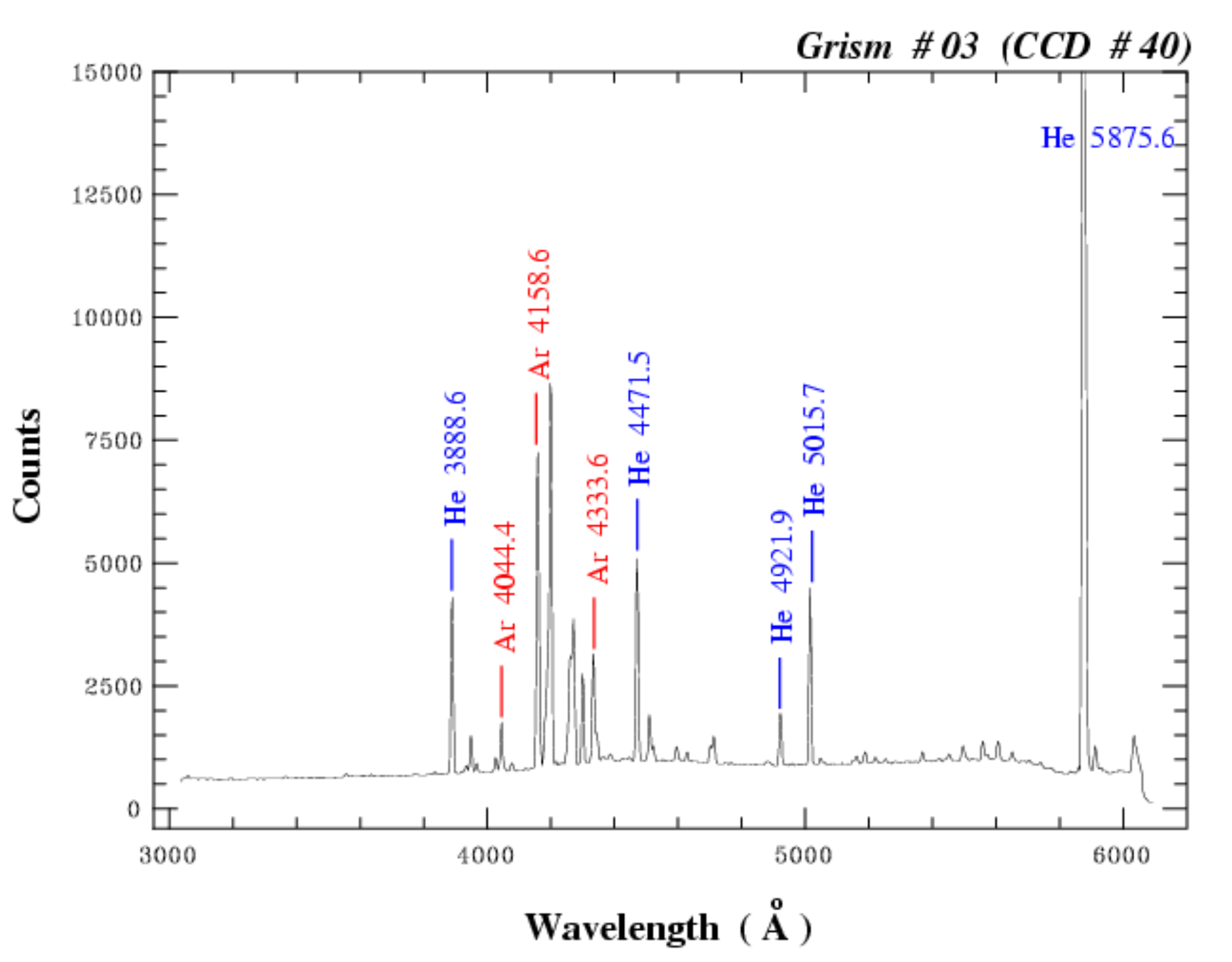
We can now pass onto identifying the emission lines of the calibration lamp. In this case the calibration lamp
contains a mixture of helium and argon gas which creates a series of emission lines in the optical wavelength range.
Make sure you have your so-called 'line map' ready. This map indicates which emission features correspond to which emission lines.
You can find the line map on ESO's instrument website for EFOSC2. I've included it below for reference:
pynot identify:
pynot identify arcs/corr_arc_frame.fits
You now have to 'add' the reference lines by moving the cursor to a given emission line and click the a key
and then input the reference wavelength in the new table entry. Note that the reference line list is given in the left-most
table of pynot identify. See more details about the line identification on the task description of
pynot identify.
When you are happy with the fitted wavelength solution you can save the pixel table to a file, such as 'pixeltable_gr3.txt'.
We can now apply this wavelength solution to the first science image in order to 'rectify' the image,
that is, apply the wavelength solution to each column of the image (as these are dipersed vertically).
We do this step using the task pynot wave2d.
pynot wave2d science_file.fits arcs/corr_arc_frame.fits --table pixeltable_gr3.txt --output wavecal_science.fits
We have now created the wavelength calibrated image 'wavecal_science.fits' together with a diagnostic plot of the fitted
2D wavelength solution in the PDF file: PixTable2D.pdf. This file should show the arc calibration image
with the traced position of the emission lines along the spatial direction. Also check that the residuals around each
identified emission line are small. If things go wrong here, consult the details of the task,
pynot wave2d.
The instrument response function
First step in determining the instrument response is to apply the wavelength calibration to your standard star observation
that we processed above.
This is done the same way as in the previous step using the task pynot wave2d.
After the 2D data have been wavelength calibrated, we can extract the 1-dimensional spectrum of the standard star.
We will do this using the task pynot extract. You can follow the steps
of that task using the previous link. Make sure to give the 1D spectrum a sensible filename, such as 'EG21_1D.fits'.
Last step in determining the instrument response function is to compare the number of counts received on the detector as a
function of wavelength to the known flux of the standard star.
The list of standard stars that PyNOT knows about is given on the pynot response page.
These stars have very well-measured fluxes at specific wavelengths making them ideal fluc calibration references.
We calculate the response function by using the task pynot response:
pynot response wavecal_EG21_1D.fits --output response_gr3.fits
Cosmic ray rejection
The best way to reject cosmic rays is to combine multiple exposures but if you only have one exposure
with a lot of cosmic ray hits you can flag and interpolate over these using the task
pynot crr:
pynot crr science_file.fits --output crr_science_file.fits
objlim and sigclip.
What happens if you lower these thresholds?
The rejection step keeps track of what pixels were flagged and stores these in a separate mask extensions of the output FITS file. In this mask, values of 0 mean good pixels, and pixels with values 1 are bad. This mask image will be used in further steps for the spectral extraction to exclude pixels in the extraction or image combination.
Flux calibration
As of now, we have corrected the detector artefacts (bias and flat-field corrections)
and calibrated the wavelength solution. We therefore have a 2-dimensional image with wavelength increasing
positvely (left-to-right) along the horizontal axis, and spatial position (in pixels) along the slit along the
vertical axis. However, the data remain in units of counts (or ADUs) integrated over the whole exposure.
The last step in the data carlibration is therefore to convert these counts to physical flux density units.
This is where the response function, that we just calculated, comes in handy.
There are two ways to apply this flux calibration:
-
flux calibrate the 2-dimensional image such that each pixel
has a unit of flux density (per spatial pixel) and then extract a 1-dimensional spectrum from this image,
using the task
pynot flux2d; -
or firstly extract the 1-dimensional spectrum from the image and then apply the flux calibration
to the 1-dimensional spectrum, using the task
pynot flux1d.
pynot flux2d task to calibrate the image that was corrected for cosmic
ray hits:
pynot flux2d crr_science_file.fits response_gr3.fits --output science_2D_final.fits
Note: It's a good idea to test your flux calibration by applying it to the standard star spectrum itself. For this,
we use the pynot flux1d task as we already extracted the total
flux of the standard star. Try to find a reference spectrum of the standard star online (a google search should be enough).
How does this compare to the flux calibrated spectrum of the standard star that you have calculated here?
Sky subtraction and object extraction
We are now ready for the final step in the data reduction process, namely the spectral extraction. Due to dispersion by the instrument optics and most notably due to the seeing induced by the atmosphere, the flux from our objects does not land on a single row of pixels on our detector. Instead the light is spread out along the slit. This spread is what we will refer to as the "spatial profile" or the spectral PSF (SPSF, which is 1-dimensional compared to a 2D image PSF). In this step, our goal is to sum up all the flux from the object which has been spread out according to this SPSF. There are a few ways of doing this, and the simplest way is simply to define an extraction aperture along the slit and sum up all the pixels in that range. This will add all the flux but also add a lot of noise from regions that are dominated mostly by the sky-background. Instead, we can use a more efficient algorithm called the "optimal extraction", where we apply a weighting of each pixel according to how much flux that given pixel should receive in agreement with the SPSF. For details, see Horne 1986.
PyNOT allows you to perform the extraction using an interactive graphical interface which also allows you to determine
the sky background level (if enough clean sky regions are observed along the slit) and subtract it before extracting your object
spectrum. For more details, see the dedicated page of the pynot extract task.
You can run the extraction software with the following command:
pynot extract science_2D_final.fits