For more information about me and my research, visit my homepage:
PyNOT : skysub
This task takes a 2-dimensional image as input and performs a background subtraction using an automated object detection and masking. The background level is then fitted by a polynomial of variable degree excluding pixels flagged as objects (i.e., significantly above the noise level) or artefacts such as cosmic rays. The task performs the following sub-tasks:
Object detection
The object detection is performed by first collapsing the data array along the dispersion axis to obtain the
spatial profile along the slit. If the dispersion axis is incorrectly identified from the file itself
you can set it using the --axis option. Next, the noise level is determined based on the median
absolute deviation (MAD) of the data themselves. Objects are then identified as peaks in the spatial profile
above a certain threshold defined as \( \kappa_{\rm obj} \times {\rm MAD} \) using scipy.signal.find_peaks.
The threshold factor is set to 20 by default but can be changed by the --obj_kappa option.
Additionally, a peak must extend over at least 3 pixels to be considered a real object. The width of each peak
estimated and used to mask out pixels around the centroid: \( x_{\rm cen} \pm s \times {\rm width} \), where s
is a user-defined scale-factor (by default set to 3). The scale-factor can be changed by the --fwhm_scale
option. The object detection algorithm is illustrated in Fig. 1.
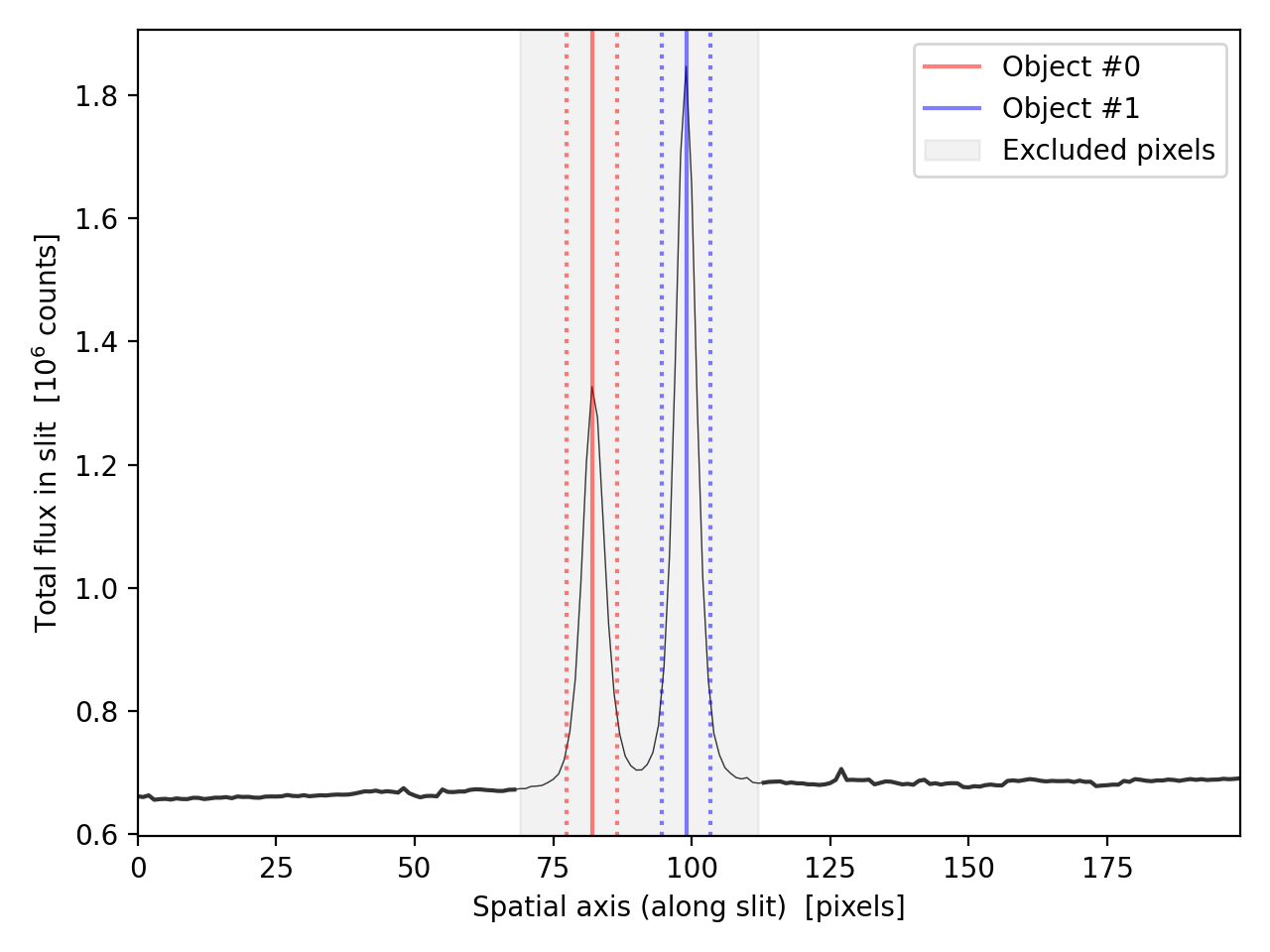
pynot skysub algorithm has automatically
identified the two objects marked by the solid vertical lines of different color. The dotted lines on either side
of the solid line indicated the estimated FWHM of the object used to define the masking region.
The gray shaded region indicates the exclusion region around the objects as identified by the code.
Note: This algorithm has been optimized for point sources or objects which have significant amount of empty background within the slit. Very extended objects may require a different strategy, such as "Nodding along the slit" or "Offset sky observations". PyNOT does not currently handle such strategies. You can also use the interactive tool pynot extract to determine a background model, subtract it and save the result.
Polynomial fitting of rows (wavelength bins)
Once any objects have been identified, the code loops through all the rows of the data array, that is, each wavelength bin
along the dispersion axis is fitted idenpendently. It is therefore recommended to apply a 2D rectification of the dispersion
axis along the slit using pynot wave2d. This ensures that skylines are straightened out.
Any residual "curvature" of the sky-lines may lead to residuals in the sky-subtracted image.
Each row is filtered using a median filter in order to clip artefacts, such as cosmic ray hits or bad pixels.
The noise-level per row is determined using the MAD, and outlying pixels are flagged if they are more than
\( \kappa \times {\rm MAD} \) above or below the median filtered row. The options of the median-filtering and sigma-clipping
are controlled by the options --med_kernel and --kappa, respectively.
Lastly, the pixels that are not flagged as objects, outliers and fall within the --xmin and --xmax values
are used to fit a Chebyshev polynomial of variable degree, controlled by the option --order_bg. By default
a 3rd order polynomial is used. The xmin and xmax values are used to exclude any artefacts at the edge
of the data array (CCD artefacts, vignetting, etc).
An example of the fitting algorithm is shown in Fig. 2.
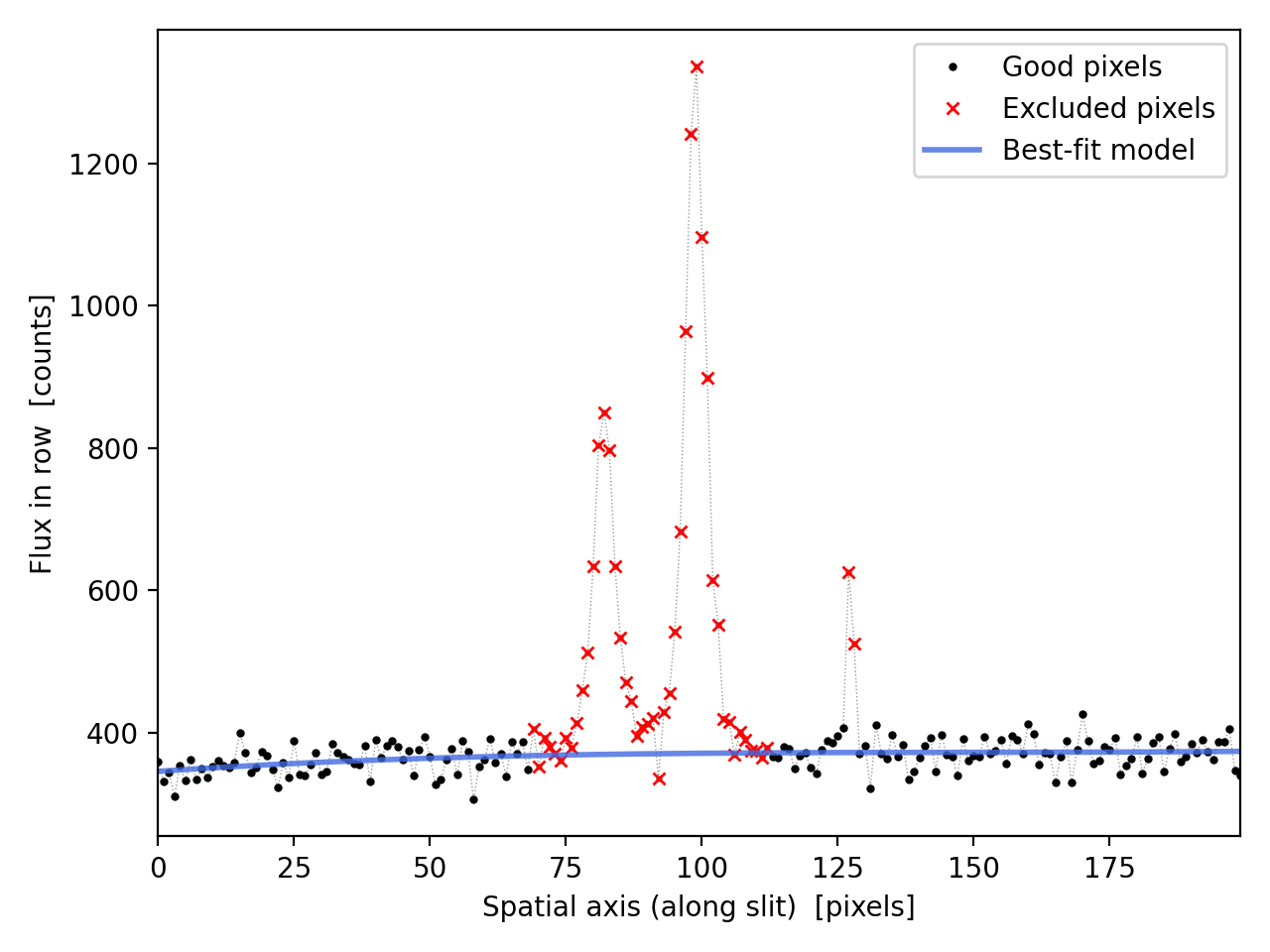
pynot skysub algorithm has automatically
identified the outlying pixels caused by a detector artefact (the spike on the right-hand side of the two objects).
Excluded pixels are highlighted as red crosses whereas black dots mark the good points used for fitting
the polynomial. The best-fit background model is shown as the thick blue line.
Saving the output:
The output from pynot skysub is saved as a FITS file with an added extension named "SKY"
which holds the 2D background model subtracted from the science image. The filename must be given with the --output
(or -o) option in the command line.
Example Syntax
pynot skysub -o OUTPUT input
Full example of command line syntax:
pynot skysub [-h] -o OUTPUT [--axis AXIS] [--auto AUTO] [--order_bg ORDER_BG] [--kappa KAPPA] [--med_kernel MED_KERNEL] [--obj_kappa OBJ_KAPPA] [--fwhm_scale FWHM_SCALE] [--xmin XMIN] [--xmax XMAX] input
Overview of parameters
- input
- Input filename of 2D frame
- --output (-o)
- Output filename of sky-subtracted 2D image [REQUIRED]
- --axis: 2
- Dispersion axis: 1 horizontal, 2: vertical
- --auto: True
- Automatically subtract the sky from the 2D spectrum?
- --order_bg: 3
- Polynomial order for sky background subtraction (per row)
- --kappa: 10
- Threshold for rejection of outlying pixels (cosmics etc) in units of std. deviations
- --med_kernel: 15
- Median filter width for defining masking of cosmic rays, CCD artefacts etc.
- --obj_kappa: 20
- Threshold for automatic object detection to be masked out.
- --fwhm_scale: 3
- Mask out auto-identified objects within ±`fwhm_scale`*FWHM around centroid of object
- --xmin: 0
- Mask out pixels below xmin
- --xmax: None
- Mask out pixels above xmax