For more information about me and my research, visit my homepage:
PyNOT : identify
Calibrations require knowledge of the instrument
The instrument manual usually includes a list of so-called arc line atlases that show how the arc lines of the various calibration lamps look using the available dispersive elements (mainly grisms). These atlases also indicate the reference wavelengths of most if not all prominent lines in the setup. Make sure you have the appropriate line atlas available for the setup you're reducing.
Getting started: Loading Data
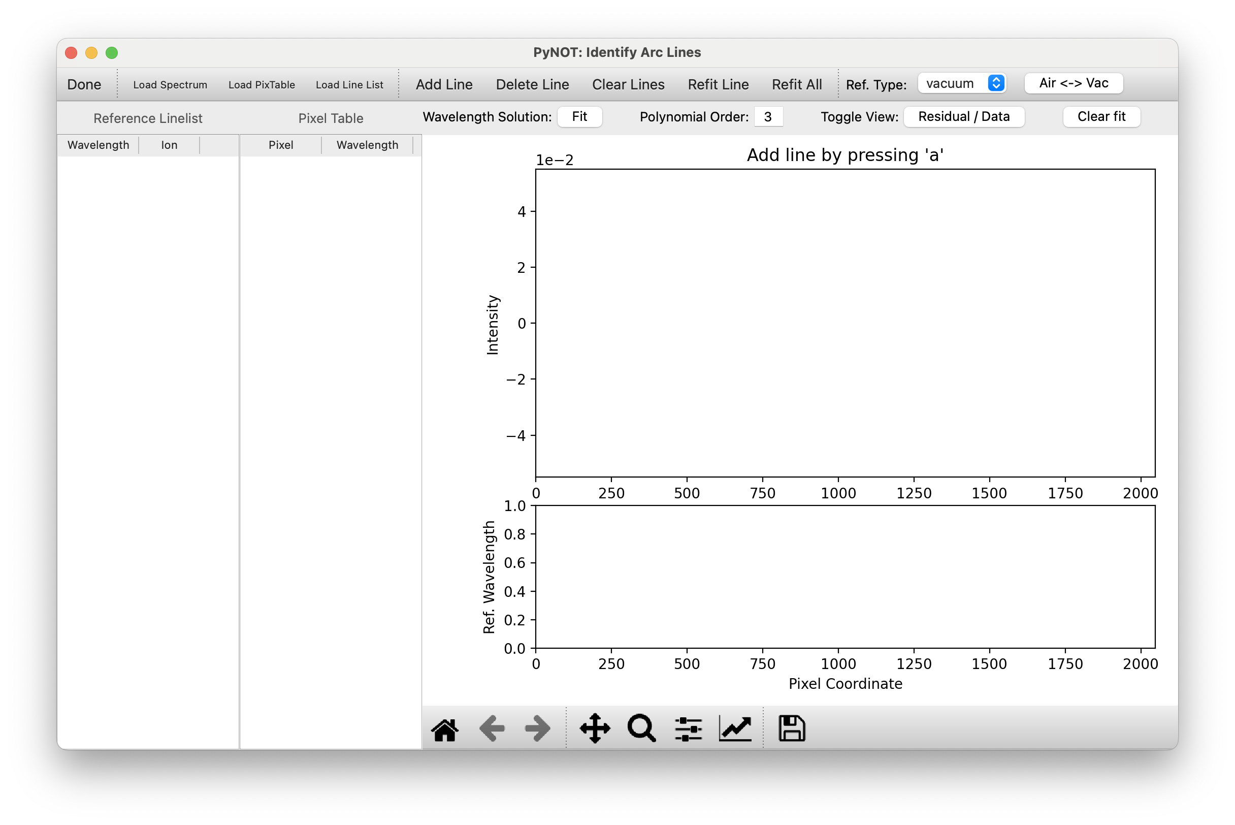
The first step of the wavelength calibration is to identify the wavelength of known emission lines. This is done in an interactive window launched when running the taskpynot identify. This will open a blank
window as seen in Fig. 1. You can now load the arc-line image (bias-subtracted using pynot corr for better results).
To load the calibration image, select "Load Spectrum" from the File Menu or use the button "Load Spectrum".
You can also run this task with an input arc-line calibration image directly from the command line.
pynot identify.
The arc line spectrum will be extracted at the center of the slit by default. Otherwise use the
--loc option
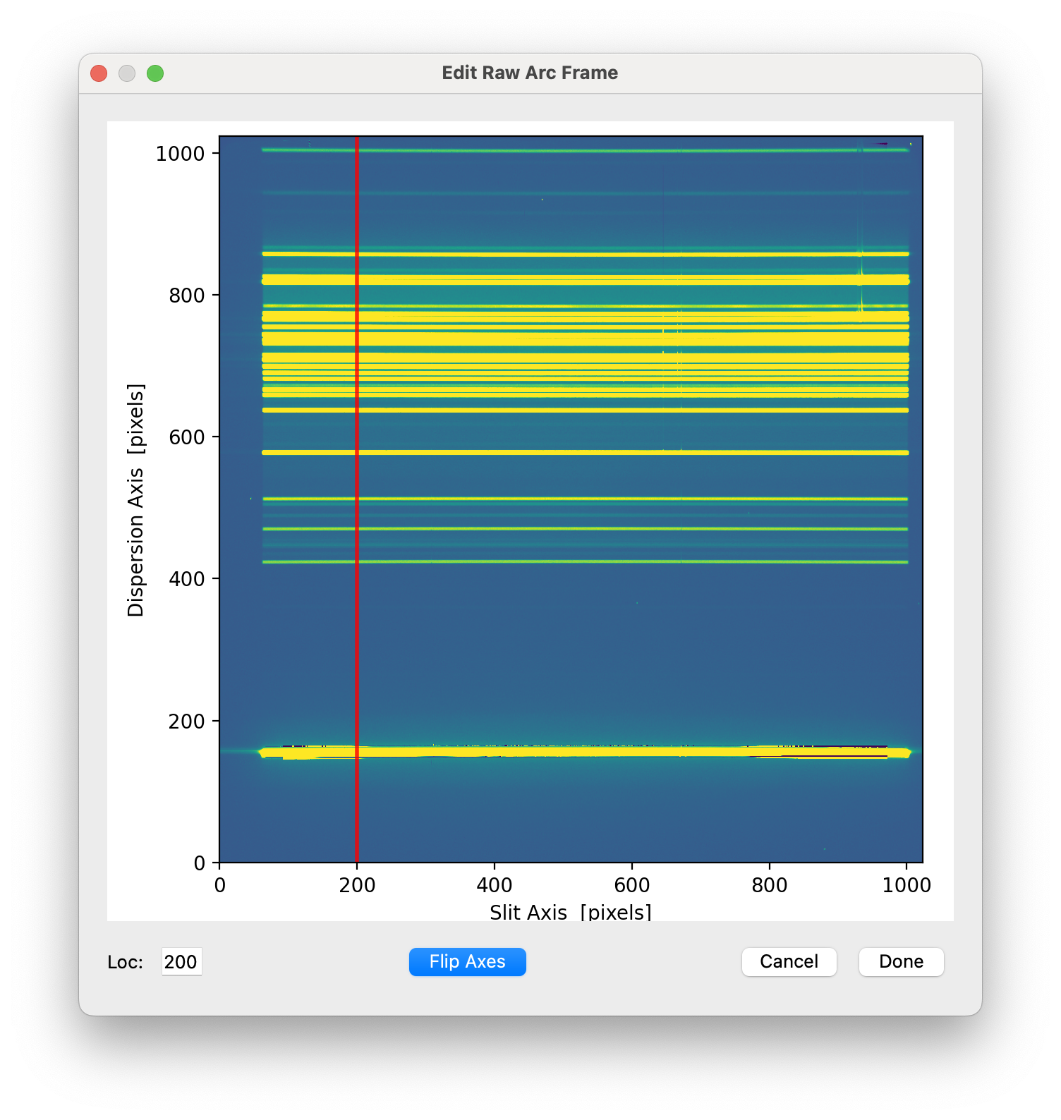
from the command line to set the pixel location along the slit, or select "Set 1D Location" from the File Menu (see Fig. 2).
The extraction location is shown by the thick red line and can be changed in the input field 'loc' in the bottom left corner.
If the spectrum is not oriented correctly, i.e., the dispersion axis has not been identified correctly, you can flip the axes
to ensure that the extraction of the calibration lines is done correctly.
Identifying Lines
If a wavelength solution already exists from a previous reduction of the same spectral setup, you can load the pixel table (the output generated by pynot identify) if it's not automatically loaded. If you are starting from zero, you will have to:- Load the reference line list (if not automatically loaded by PyNOT) using the "Load Line List" button. This line list should match the calibration lamp used in your observations (typically HgNe or ThAr). This will populate the left-hand table in the window.
-
Add lines one by one either by pressing the
Akey or clicking the "Add Line" button. The main plotting window on the right-hand side will now tell you to click on the emission line that you want to identify. It can be helpful to zoom in to make sure you hit the right line. The line position will then be fitted using a modified Gaussian to allow for the slightly flattened line-shape that is typically observed for bright calibration lines. Note: Make sure you have your line atlas handy for the given spectral setup! You can usually find this on the observatory/instrument website. - The line position in pixel space will be added to the middle table showing the "Pixel Table". This table is the basis of the wavelength calibration, i.e., the translation from pixel space along the dispersion axis into wavelength space. You will be prompted for the corresponding wavelength which will have to be one of the reference wavelengths in the left-hand table. Note: You don't have to give all the decimal points unless there are two lines very close to each other. The code will automatically look-up the matching reference wavelength closest to the value you input.
- Keep adding lines until you have identified at least 5 or 6 lines over the full wavelength range. The final result should look something like Fig. 3.
-
If you made a mistake with a line, you can delete it by pressing the "Delete Line" button and then clicking on the
red dotted line in the main plotting window. You can also refit a line by pressing the
Rkey while hovering the cursor over a line. This will higlight the given line as a solid red line and you can now move the cursor to the new starting guess for the centroid and pressRagain. The dotted line should now shift to the new position.
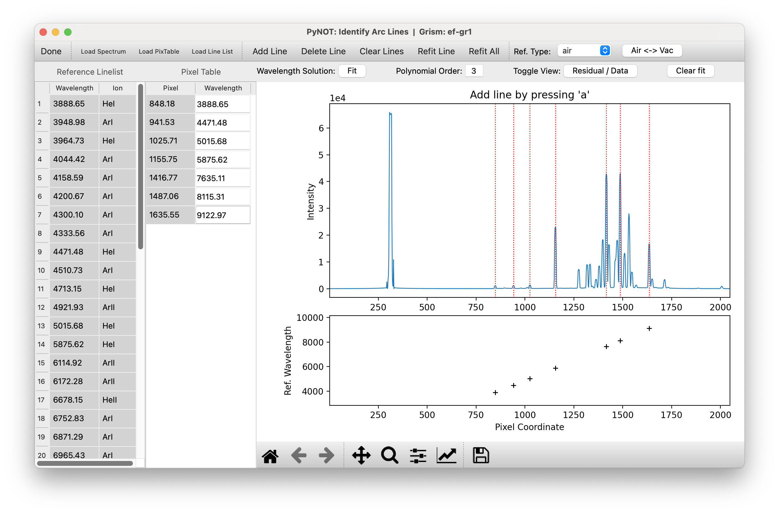
pynot identify with a set of identified
calibration lines marked by the dotted vertical lines.
Fitting the wavelength solution
After identifying a set of lines, the next step is to fit the wavelength solution using a polynomial of variable degree. By default, an order 3 Chebyshev polynomial is used. The order can be changed in the input field "Polynomial Order in the tool bar above the main interactive plotting panel. Pressing theENTER key or clicking the "Fit" button
will update the fit and show the best-fit relation between pixel value and wavelength as the solid blue line in the bottom plotting panel.
The standard deviation of the fit residuals is shown in the bottom plot to give an indication of the wavelength accuracy of the calibration.
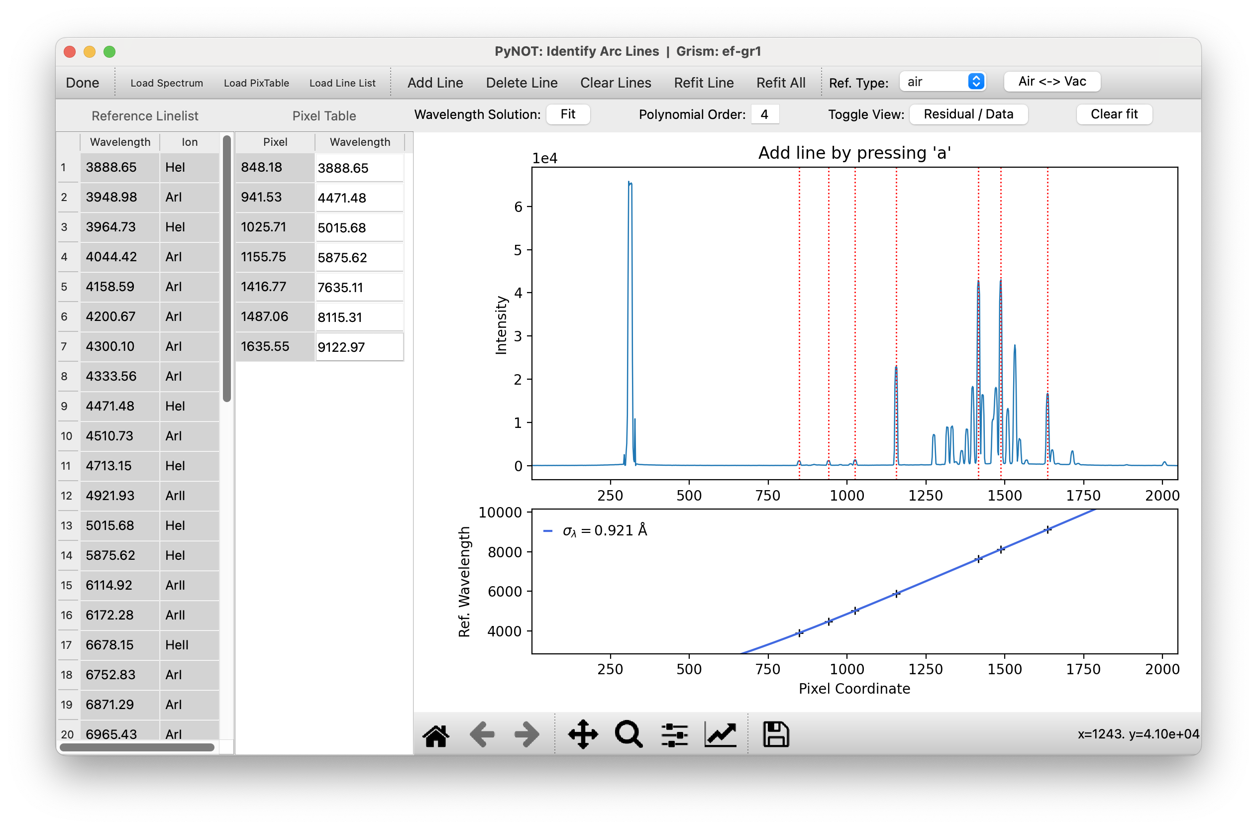
pynot identify with a fitted wavelength
calibration shown by the blue line in the bottom panel.
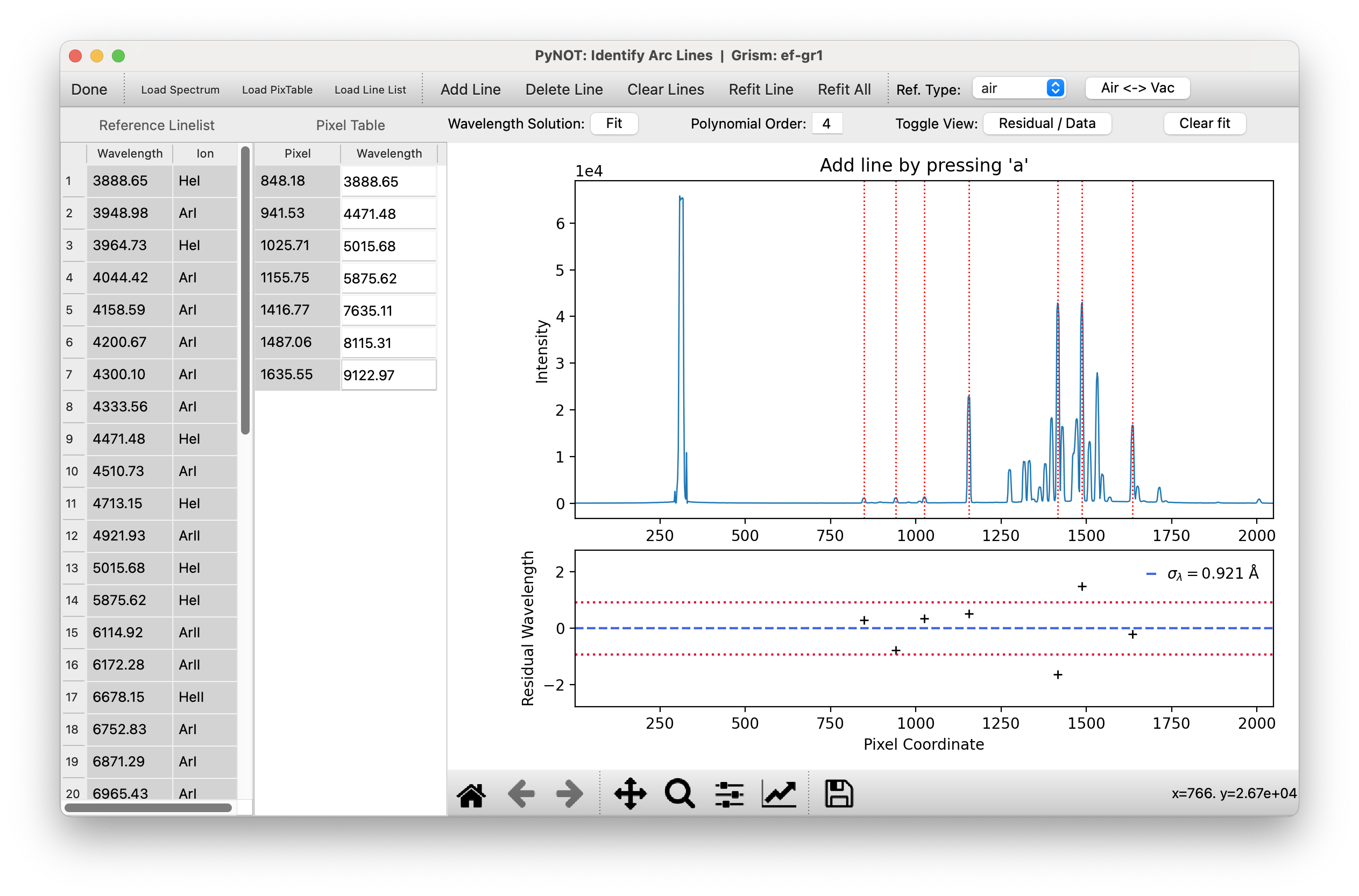
pynot identify with a fitted wavelength
calibration showing the fit residuals instead of the actual solution. Any systematic trends in the residuals would
indicate a poor fit or incorrectly identified lines.
Air or Vacuum??
Most observatories will give their calibration line lists in air wavelengths, but pay close attention to whether your reference line list is using vacuum wavelengths (i.e., corrected for the refractive index of the atmosphere). You can change the reference type in the drop-down menu "Ref. Type" in the top tool bar. This determines the system used in the loaded reference table. You can also toggle between air and vacuum wavelengths in your derived solution by hitting the "Air - Vac" button.
Saving the solution
When you are happy with the wavelength solution, you can save it by clicking "Done" in the upper left corner. This will open a dialog window allowing you to chose a filename and filepath. The solution will also be cached in the PyNOT install directory for future use of the same setup. The format of the so-called pixel table is a simple ASCII table with a few header lines commented out by the# character.
Example Syntax
pynot identify
Full example of command line syntax:
pynot identify [-h] [--lines LINES] [--axis AXIS] [-o OUTPUT] [--air] [--loc LOC] [arc]
Overview of parameters
Optional Arguments:- arc
- Input filename of arc line image
- --lines: ''
- Linelist, automatically loaded if possible
- --axis: 2
- Dispersion axis: 1 horizontal, 2: vertical
- --output (-o): ''
- Output filename of arc line identification table
- --air: False
- Use air reference wavelengths
- --loc: -1
- Location along the slit to extract lamp spectrum [pixels].