For more information about me and my research, visit my homepage:
PyNOT : wave2d
This task will take a science image and apply a transformation to remove image distortions along the spatial axis.
These distortions are most visible in the associated arc line image where the emission lines of the calibration lamp
show up as curved lines instead of straight lines. The task wave2d performs the following sub-tasks:
- Image edge detection
- Arc lamp continuum subtraction
- Arc line fitting: the 2D pixel table
- Image transformation and wavelength linearization
- Overview of parameters
Image edge detection
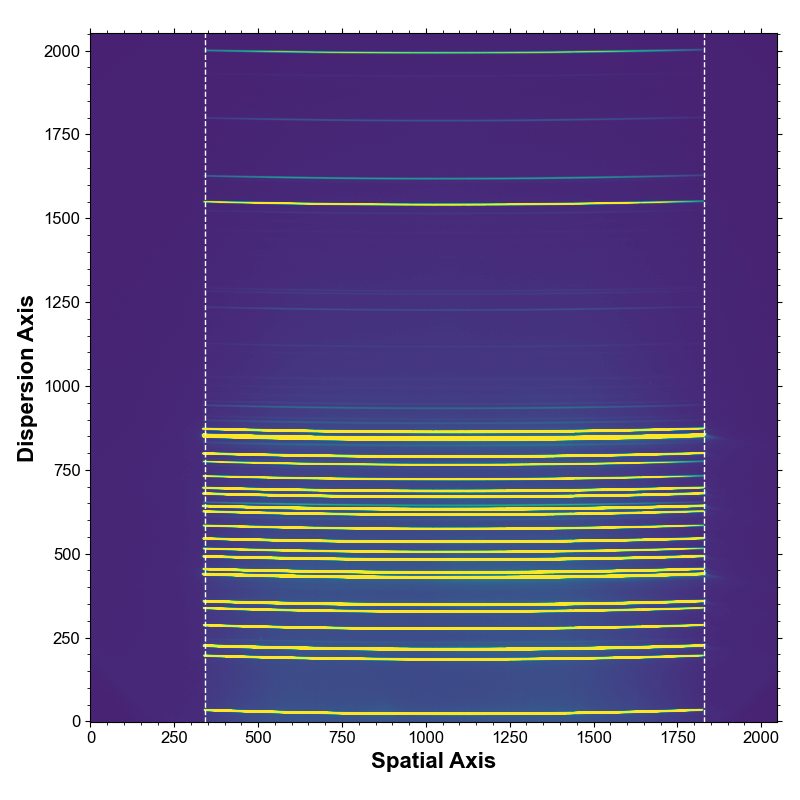
The first step in the process is to detect the edges of the exposed region of the image. This is done by finding the
location along the slit where the arc lines are no longer visible. This is illustrated in Fig. 1, where the significant
curvature of the arc lines is visible as well. The edge detection is controlled by the single parameter edge_kappa.
This parameter determines the significance level above which the emission lines must be detected.
If the emission lines are very weak at the edge, it might be necessary to lower this threshold in order to detect the fainter edges.
Setting this parameter too high might result in an aggressive rejection of all emission lines, and hence a very unstable edge detection.
Note that for images where only the central part of the CCD has been read out, this step is not technically necessary but it allows the user to identify cases where the arc lamp illumination failed during the calibration exposure, or other glitches.

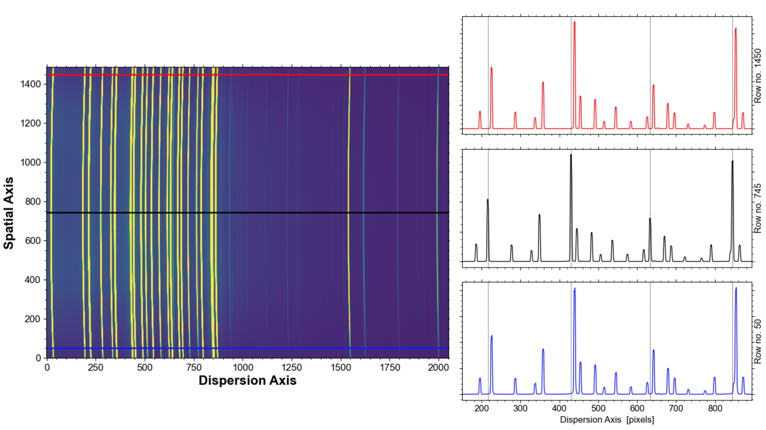
The arc and science images are then trimmed and rotated to have dispersion along the horizontal axis. This is done to speed up the calculations, as operations on rows in Python are slightly faster than operations by columns. The resulting trimmed arc image is shown in Fig. 2 together with examples of spectra along three rows (one at either end and one in the middle).

Arc lamp continuum subtraction
Now that the arc line image has been trimmed, we can start to fit the positions of the emission lines for each spatial row.
But before the emission lines are fitted, the smoothly varying lamp continuum is subtracted in order not to bias the measurements
of the line positions.
The lamp continuum is estimated for each row by masking out the emission lines using a median-filtering procedure. The resulting
continuum regions are then interpolated using a Chebyshev polynomial of order given by the parameter order_bg.
Lastly, the continuum estimate is subtracted from the given row.
Arc line fitting : the 2D pixel table
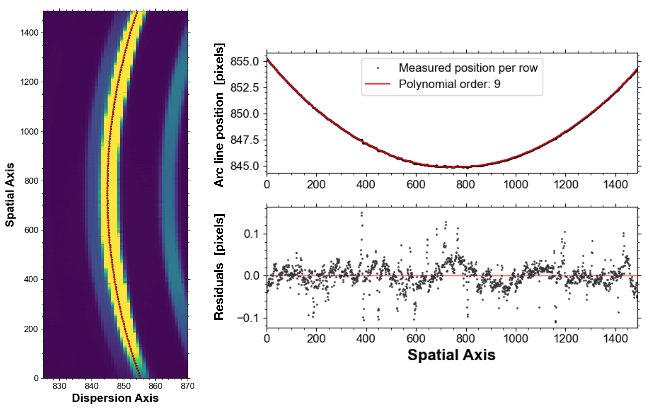
For each arc line identified by PyNOT-identify the task now fits the location of the given emission line for each spatial row.
This is illustrated in Fig. 3 for one emission line. The line center is obtained by fitting a Gaussian to the predicted position
from the input pixel table (given by the required argument table). The fit is performed in a small region
around each line, by default a region of 10 pixels on either side is used. This region can be controlled by the parameter
fit_window.
Note: if many of the identified arc lines are close together (i.e., within the fit_window) the fit may fail
silently since the stronger of the emission lines will always be fitted. This leads to degeneracies in the subsequent
calculation of the wavelength grid. One way to see this, is if the wavelength residuals are very large. In some cases
the code will fail with an error that the wavelength solution is not monotonic. This is most likely a result of arc line
identifications that are too closely spaced or a fit_window that is too wide.
The fit_window must, however, be wide enough such that the maximum curvature of the arc line falls within the
fitting region. The 'maximum curvature' is printed in the log after the fitting.
The fitted positions are then median filtered and fitted by a Chebyshev polynomium as a function of the spatial pixel value
(top right panel of Fig. 3). The polynomial order used is controlled by the parameter order_2d. The fitted
polynomium is then used to calculate the predicted position for each spatial row (red line in Fig. 3).

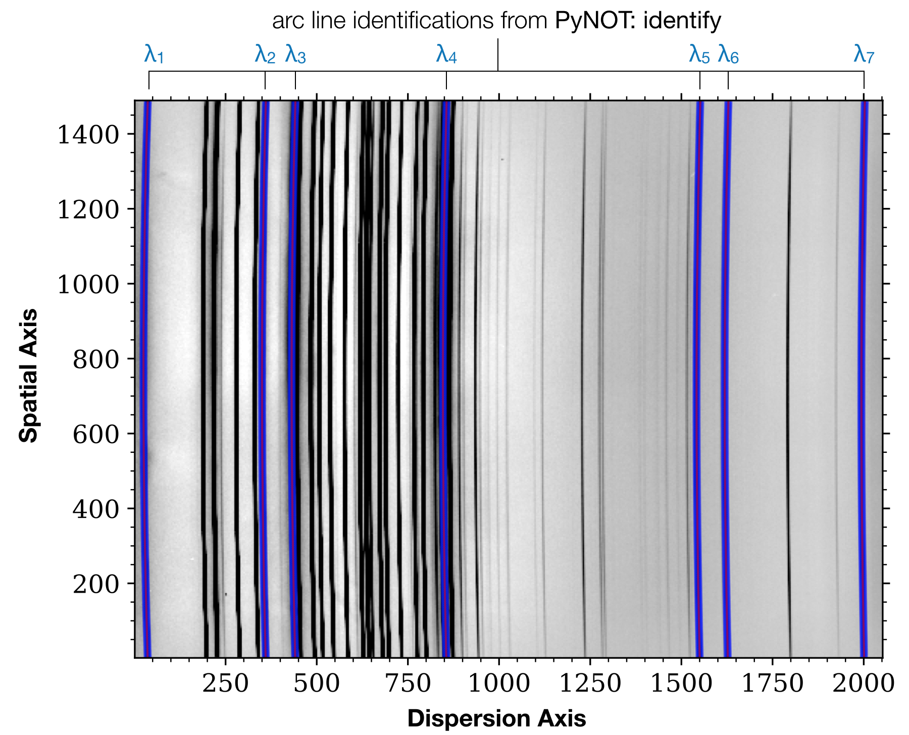
These predicted positions are obtained for each arc line in the pixel table generated by PyNOT-identify. The result after this subtask is a 2-dimensional pixel table where each identified arc line has been traced along the spatial rows. The 2D pixel table is overplotted on the trimmed arc line image and saved as a diagnostic plot. It is a good idea to inspect this plot to verify that all arc lines have been traced correctly. One example of such a 2D pixel table is shown in Fig. 4.

Obs! If the input arc line image has been over- or under-exposed, the automated line tracing may fail. You should always make sure that the arc line images have been appropriately exposed. If there's a large contrast between bright and faint arc lines, or if the illumination towards the slit edge is too poor, it might be necessary to combine several arc line images taken with the same slit.
Image transformation and wavelength linearization
The wavelength solution at each spatial row is then obtained as:
\( \lambda_i (x) = C_{\tt order\_wl}(x\ |\ \lambda_{\mathrm{ref}}, x_{{\rm ref}, i}) \)
where \(C_{\tt order\_wl}\) refers to a Chebyshev polynomium of order determined by the parameter order_wl,
given the interpolation reference wavelengths, \(\lambda_{\rm ref}\) and the arc line position for the given row, \(x_{{\rm ref}, i}\)
(see above).
In order to rectify the science frame, each row along with its associated error and quality mask is now interpolated
onto the reference wavelength grid. The central row is by default assumed as the reference position. Hence, all other
rows will be aligned to the wavelengths defined by the central row (or whatever row was used to identify the arc lines).
Values that fall outside the reference wavelength grid are set to 0.
Example Syntax
pynot wave2d --table TABLE -o OUTPUT input arc
Full example of command line syntax:
pynot wave2d [-h] --table TABLE -o OUTPUT [--axis AXIS] [--order_wl ORDER_WL] [--order_bg ORDER_BG] [--order_2d ORDER_2D] [--log LOG] [--N_out N_OUT] [--interpolate INTERPOLATE] [--fit_window FIT_WINDOW] [--plot PLOT] [--edge_kappa EDGE_KAPPA] input arc
Overview of parameters
- input
- Input filename of 2D spectrum
- arc
- Input filename of arc line image
- --table
- Pixeltable of line identification from 'PyNOT-identify' [REQUIRED]
- --output (-o)
- Output filename of rectified, wavelength calibrated 2D image [REQUIRED]
- --axis: 2
- Dispersion axis: 1 horizontal, 2: vertical
- --order_wl: 5
- Order of Chebyshev polynomium for wavelength solution
- --order_bg: 5
- Polynomial order for background subtraction of calibration lamp continuum
- --order_2d: 3
- Polynomial order for spatial reconstruction of arc lines
- --log: False
- Use logarithmic binning in wavelength?
- --N_out: None
- No. of output pixels along dispersion axis. If null is given, use No. of pixels in input image.
- --interpolate: True
- Perform interpolation or apply central wavelength solution to full 2D range
- --fit_window: 10
- Fitting window in pixels around each arc line to determine centroid (optimized for grism 4)
- --plot: True
- Make diagnostic plots?
- --edge_kappa: 10
- Significance threshold for edge detection of arc lines