For more information about me and my research, visit my homepage:
PyNOT : sflat
This task will take a series of calibration exposures taken with a continuum lamp. These should use the
same spectroscopic setup as your science exposures (same slit and dispersive element).
The goal of this task is to remove artefacts in the data caused by variations in the detector
effeciency as well as impurities in the optical path.
The task sflat performs the following sub-tasks:
Combination of spectroscopic flat-field calibrations
The first step of the task pynot sflat is to remove the bias level and overscan regions
of all the individual spectroscopic flat-field exposures. For this prupose, a combined bias image
must be provided using the command line option --bias.
After the bias level has been removed, the different flat-field exposures are combined using
a sigma-clipped mean combination by default. The threshold for the sigma-clipping can be controlled
by the parameter --kappa. You can also chose to perform a median combination by
setting the parameter --method median. The resulting combined flat-field will be saved
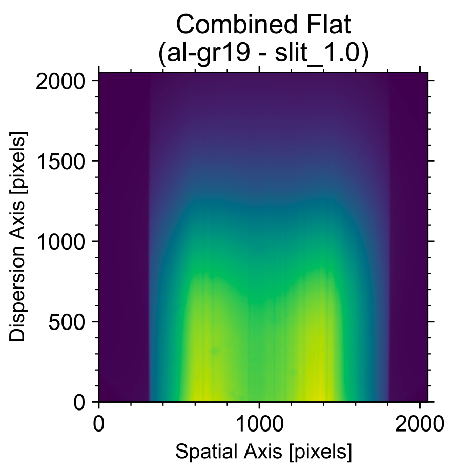
to a FITS file which by default is named after the slit width and dispersive element. An example
is shown in Fig. 1:

- The two sharp edges indicate the edges of the grism which are blocking part of the CCD;
- The spatial variations with two peaks is an artefact of the calibration lamp not illuminating the slit evenly;
- And lastly, the spectral variation (along the vertical axis) is due to the combination of the intrinsic spectral shape of the continuum lamp and the instrument throughput.
pynot init using the grep command:
%] cat dataset.pfc | grep SPEC_FLAT > flat_.list
You can further filter on specific setups in the file, such as slit, grism, filter, exposure time etc.
Make sure only to combine spectral flat fields taken with the same instrumental setup and detector characteristics (binning, readout mode, windowing). The code will complain if the image sizes do not match but any other checks is left for the user.
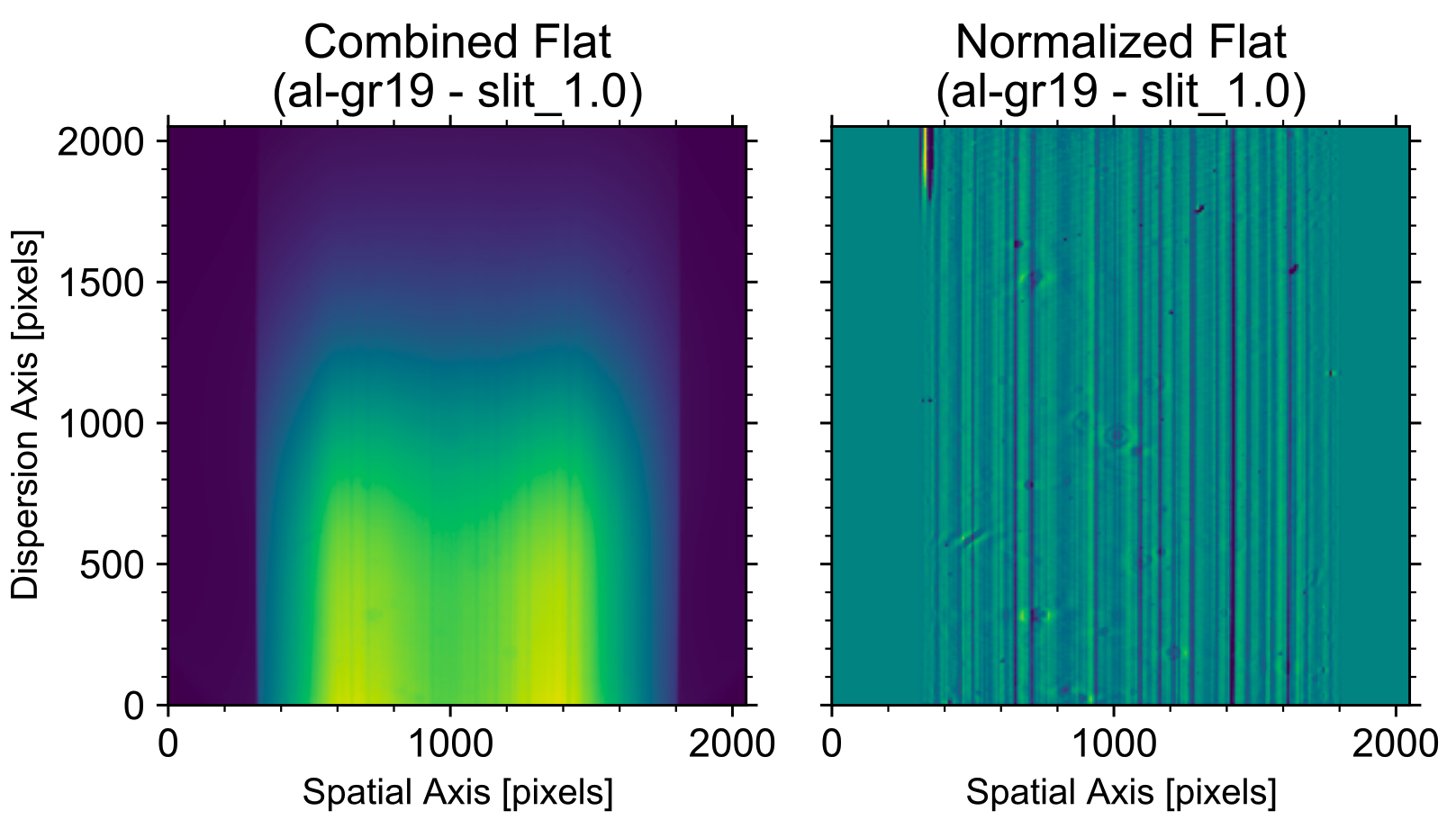
Flat field normalization
Given the non-uniform illumination of the slit by this calibration unit, we cannot use these exposure to perform an illumination correction. For this purpose, the spectroscopic flat-field exposures should be obtained using the twilight sky. However, PyNOT does not cover illumination corrections yet.Instead, we must characterize both the spatial and spectral variations in order to divide them out. This is what we refer to as normalization of the flat-field. PyNOT does this by determining the spatial profile of the flat-field in each wavelength bin using a Savitzky–Golay filtering algorithm as implemented in
scipy. The parameters of
the filtering can be controlled via the parameters --order and --savgol_window
from the command line. Before filtering and fitting the spatial profile in individual wavelength bins,
the image is first median filtered along the spectral axis to decrease the noise. A default of
5 pixels are median combined. This can be controlled using the parameter --med_window.
For more information about the parameters, run pynot sflat -h or see below.
The code determines the edges of the illuminated part of the CCD using a similar filtering algorithm and its first derivative to look for sharp features. In Fig. 1, the edges of the illuminated part of the CCD are clearly visible.
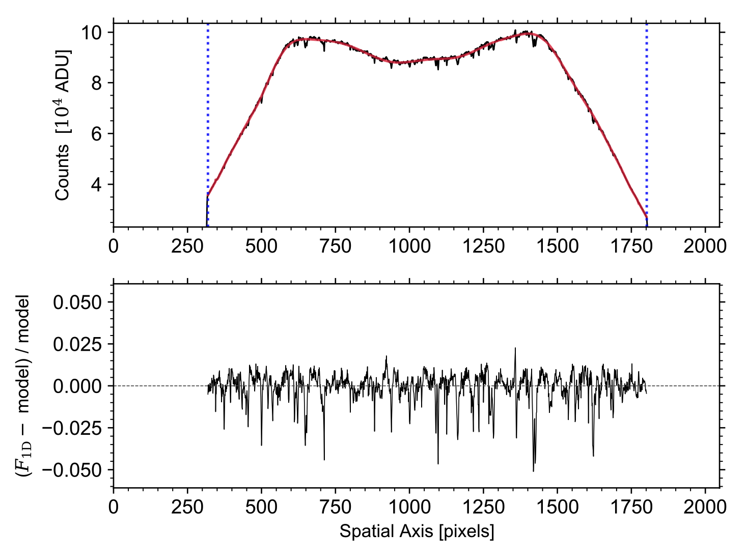
An example of the normalization of the spatial profile is shown below in Fig. 2 below, and a similar diagnostic plot is saved to the working directory with a filename starting with 'specflat_1d'. The exact filename is given in the log when running the task.


Example Syntax
pynot sflat --bias BIAS input
Full example of command line syntax:
pynot sflat [-h] --bias BIAS [-o OUTPUT] [--axis AXIS] [--kappa KAPPA] [--method METHOD] [--order ORDER] [--savgol_window SAVGOL_WINDOW] [--med_window MED_WINDOW] [--edge_threshold EDGE_THRESHOLD] [--edge_window EDGE_WINDOW] [--edge_width EDGE_WIDTH] input
Overview of parameters
- input
- Input file containing list of image filenames to combine
- --bias
- Filename of combined bias frame [REQUIRED]
- --output (-o): ''
- Output filename of combined and normalized flat frame. Constructed from GRISM and SLIT by default
- --axis: 2
- Dispersion axis: 1 horizontal, 2: vertical
- --kappa: 5
- Threshold for sigma clipping in Flat combiniation
- --method: 'mean'
- Method for image combination (options: median/mean)
- --order: 24
- Order for Chebyshev polynomial to fit to the spatial profile (per row/col)
- --savgol_window: 51
- Window width in pixels for Savitzky--Golay filter of spatial profile
- --med_window: 5
- Window width of median filter along spectral axis before fitting the spatial profile
- --edge_threshold: 10
- The detection threshold for automatic edge detection
- --edge_window: 21
- The Savitzky--Golay window used for automatic edge detection
- --edge_width: 10
- The minimum width of peaks in the derivative for edge detection