For more information about me and my research, visit my homepage:
PyNOT : extract
This task is used to extract a 1-dimensional spectrum from the 2-dimensional detector image. The default behavior of this task is to open an interactive graphical interface which will allow you to do the following steps:
- Define extraction model or aperture
- Define sky regions
- Perform sky-subtraction
- Fit and optimize the extraction profile
- Extract the 1D spectrum using optimal or aperture extraction
- What if there are multiple objects along the slit?
The command pynot extract calibrated_image.fits takes the already calibrated image,
on which the following steps have already been carried out: bias subtraction, flat-fielding,
cosmic ray flagging, wavelength calibration, and optionally flux calibration and sky subtraction.
The task will open the following graphical interface:
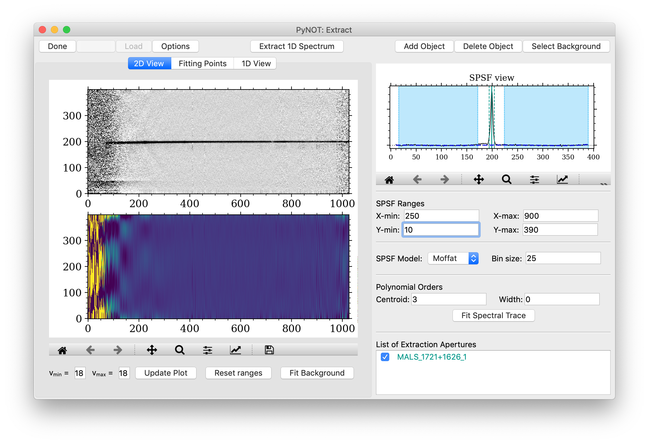
pynot extract.
The SPSF model determines how the spectrum is extracted. Using either a "Moffat" or "Gaussian"
profile will fit the SPSF along the spectral direction and use this modelled profile to perform
a weighted optimal extraction. Alternatively, the "tophat" profile can be used to perform a standard
aperture extraction by simply summing the flux within the aperture boundaries.
Adding objects along the slit:
The spectral trace denotes the location of the spectrum along the dispersion axis (for bright objects,
this is visible as a striahgt or slightly curved band in the 2D View).
The code tries to identify point sources automatically. These will be highlighted in the SPSF view
in the upper right corner as a vertical solid line.
The default width of the extraction aperture is shown by the dashed lines. The position of the center
and edges of the extraction aperture can be dragged by clicking and holding each of the lines.
Note: All extraction apertures will use the same model for the extraction: either optimal
(using Gaussian or Moffat profiles) or aperture extraction.
If the code does not correctly identify the source (or sources) you want to extract, you can manually
define a new extraction aperture using the "Add Object" button. You can then click on a position
along the slit in the SPSF viewer and the new aperture model will show up as a vertical line.
All objects are listed in the bottom part of the right-hand panel in the List of Extraction Apertues.
Right-clicking on an object in this list will bring up an option-menu which allows you to remove
or copy the aperture, as well as changing the aperture properties.
Deleting objects along the slit:
Similarly if an object has been incorrectly identified or added by mistake, you can click the
"Delete Object" button and then click on the given aperture model you want to delete.
Note: You can also drag an aperture to a new position instead of deleting and then adding
a new aperture if an object is identified at the wrong location.
Fitting the background
Next step is to define sky-subtraction regions. The automatic sky-subtraction algorithm
pynot skysub" usually does a good job but sometimes there are residual gradients
or other features in the background which can be optimized especially if there are extended objects
in the slit.
To do so, the user can select regions along the slit as background regions by clicking the button
"Select Background" or by hitting the keyboard shortcut "B". This will change the prompt
in the SPSF view and instruct the user to select the left and right borders of a sky region. This can be repeated
as many times as needed. Overlapping regions will automatically be merged.
The selected region will show up as a light blue vertical band. Sky background ranges can be removed
by clicking on the button Delete Object and then clicking on the blue band that should be removed.
The background can then be fitted using a polynomial of variable order. This is done either by clicking
the "Fit Background" or using the keyboard shortcut:
When you have selected the sky background regions, fit the background by clicking "Fit Background"
in the bottom row of the main panel or (cmd/control + shift + F). This will update the
background model view in the bottom part of the main panel and will show a model in the
'SPSF view' as a dashed blue line. The polynomial order for the background model can be changed
by pressing the "Options" button on the top row (or on mac: cmd + ,) which will bring up the
options window as shown in Fig. 2.
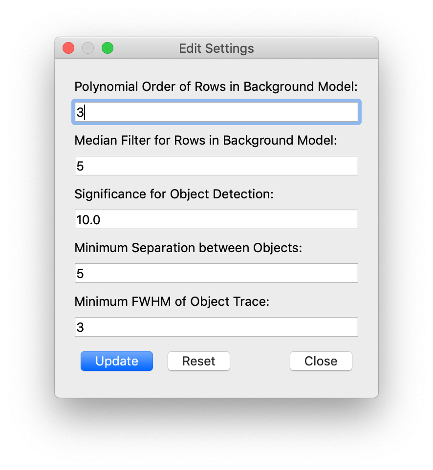
pynot extract allowing the user to
change the filtering and polynomial order used for the background subtraction. The parameters
used for the automatic object identification can also be changed.
Fitting the Spectral Trace
The spectral trace is fitted using a parametric model of the spatial profile in bins along the
dispersion axis (you change this Bin Size below the SPSF View).
There are 2 options for the parametric SPSF model which subsequently determine the profile
for the optimal extraction: Moffat or Gaussian. For a standard aperture extraction,
select the Tophat model (note that the centroid of the Tophat profile is fitted using a
Moffat profile).
To fit the position (and width of the trace model, if Moffat or Gaussian) click the
Fit Spectral Trace button (cmd + F).
A progress bar will then appear. If the fit is slow, try to use a narrower region of Y pixels
(Y-min/Y-max) and/or exclude the ends of the X-axis where the object may be too faint,
alternatively use a larger Bin Size.
Once the fitting is done, the program will switch to the Fitting Points tab shown in Figure 3.
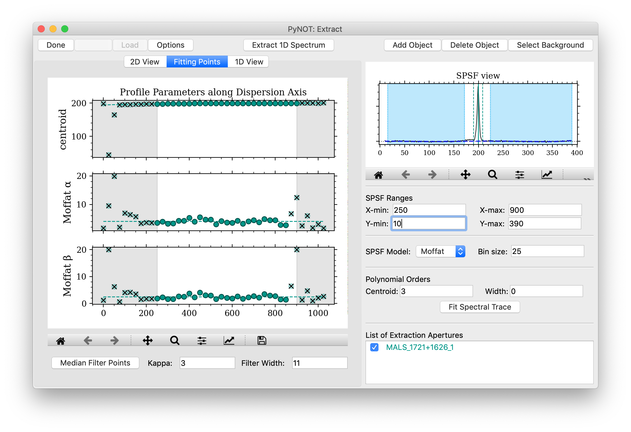
pynot extract
after fitting the spectral trace model. In this case, a Moffat profile has been fitted
along the spectral trace. The panels in this window show the fitted parameters of the model
as a function of the wavelength or pixels along the dispersion axis.
Manipulating Fitting Points:
The fitted points (solid circles) often contain outliers where the profile fit failed.
These outliers can be removed by clicking on the given point, which will change the appearance
to transparent with a black cross over it. An excluded point can be included again by clicking
on it. You can also perform a median filtering by changing the Filter Width and the
significance threshold Kappa and then clicking the Median Filter Points button.
The gray shaded regions mark the X-min and X-max limits defined in the right-hand panel.
Points in these shaded regions are excluded in the polynomial fit along the dispersion axis.
If several objects are defined you can toggle them visible/invisible by clicking on the given
tick-mark in the List of Extraction Apertures.
When you are happy with the trace model (dashed lines) along the dispersion axis,
you can verify the given profile in the 2D View, which is shown in Figure 4.
The given spectral trace will be over-plotted on the top panel
(if toggled visible in the List of Apertures).
The points shown in the 2D View can also be used to remove outlier points.
This will deactivate all parameters (centroid and widths) of the given point
(they can be re-activated under the tab Fitting Points).
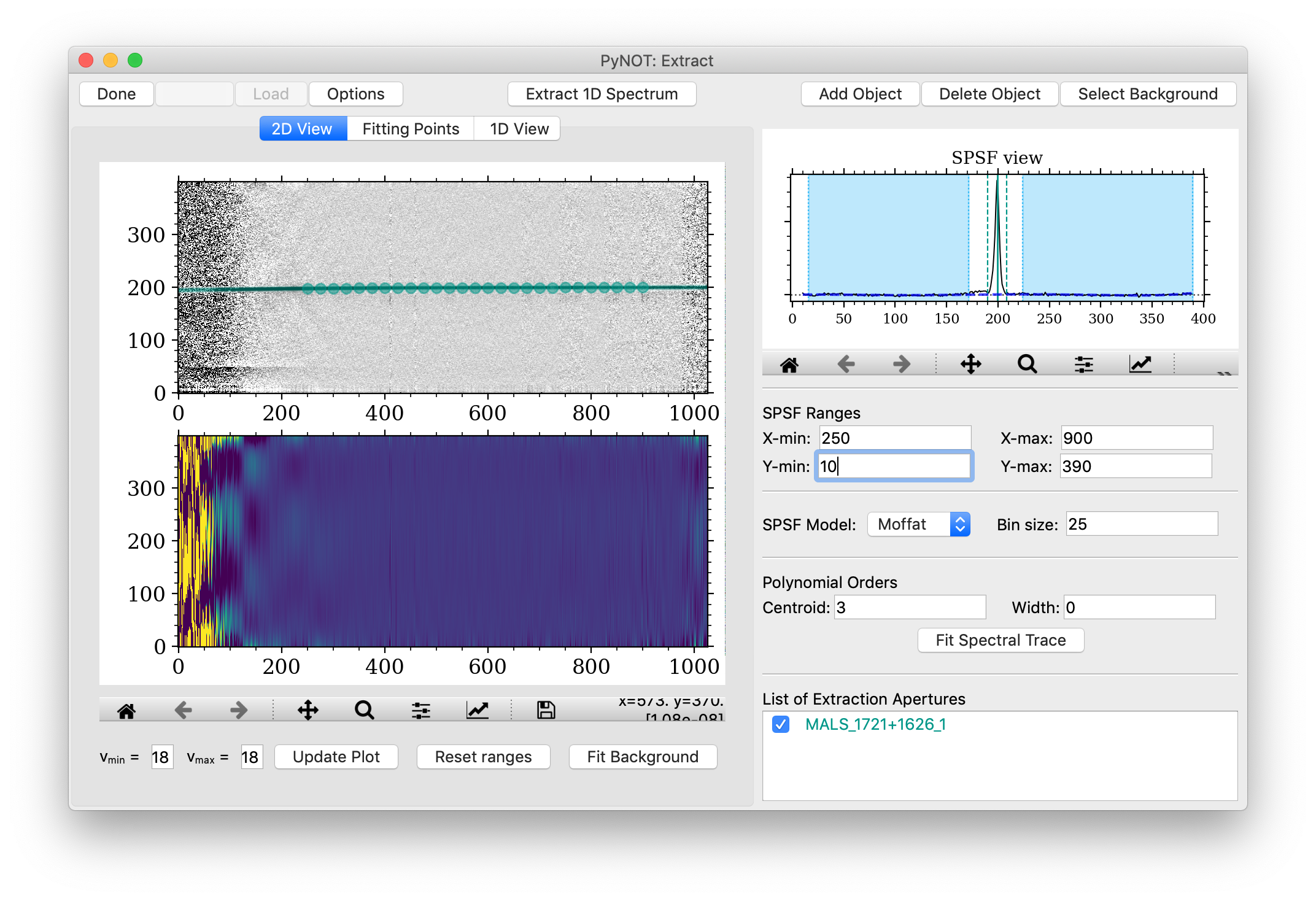
pynot extract
after fitting the spectral trace model. Here the fitted extraction aperture model is overlaid
on the science image. The points indicate the fitting points from the figure before. These can
be deselected in this view by clicking on them, see text for details.
Extracting the 1D Spectrum
When the model of the spectral trace has been defined, you are ready to extract the given aperture by clicking the "Extract 1D Spectrum" button in the middle of the top row (cmd + E). The program will change to the "1D View" tab where the extracted spectrum (or spectra, if several objects are defined) is shown, see Figure 5. The units on the X-axis (dispersion) are pixels by default, if no wavelength solution has been applied. If a wavelength solution is present, the proper units will be shown. Similar for the flux on the Y-axis, the default units are counts unless other units are present in the header of the input FITS file. The FITS Header can be shown by going to the menu: 'View > Display Header'.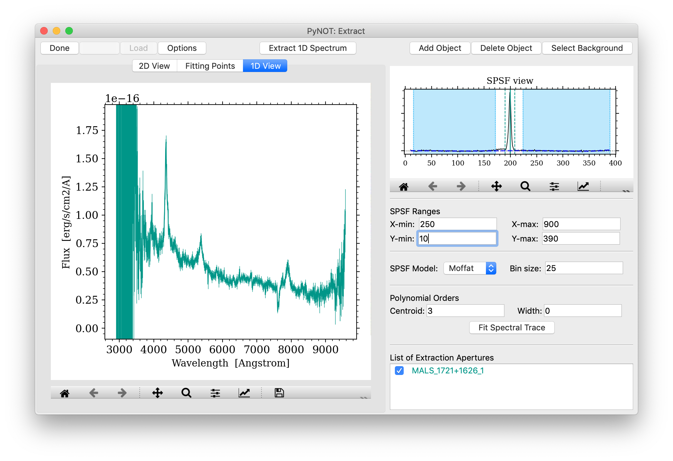
pynot extract
after extracting the 1D spectrum. Here the extracted flux is shown as a function of wavelength
or pixels along the dispersion axis, if the data have not been wavelength calibrated.
If more than one spectral aperture is defined, all spectra will be shown unless they are de-selected
in the List of Extraction Apertures by clicking the tick-box.
When you have successfully extracted the 1D spectrum and verified that it looks as expected, you can save the 1D extraction by pressing the button Done on the top row. This will promt you to save the spectrum in various formats: FITS, FITS Table or ASCII (a short example of the format is shown). If several objects are defined, you can save them all as individual extensions of a FITS Table by pressing Save All.
You can also save individual spectra by right-clicking on the given aperture model in the List of Extraction Apertures. This also allows you to save the extraction model profile. You can also save the sky-subtracted 2D spectrum and the sky model by using the File menu.
What if there are multiple objects along the slit?
You can extract multiple objects simultaneously by adding more aperture models (click "Add Object"). The steps are then the same as above. When fitting the spectral tracem the software fits a joint model of all the apertures that are defined (these are listed in the bottom-right part of the window). However, when adjusting the individual models in the "Fitting Points" view, it can be helpful to focus on one trace at a time. This can be done by switching off apertures in the bottom-right list of apertures. Clicking the tick box in front of each model will toggle them visible/invisible.
By default, if there are multiply objects, PyNOT will try to identify these automatically. However, if this automatic detection fails, it is most likely due to the object being too faint. In that case, it can be difficult to fit the spectral trace an obtain a good model. If this is the case, it can help to observe a brighter object along the slit and use this as a reference trace. You can then fit the reference object and copy the aperture model to another object. This is done by right-clicking on the reference aperture model and select, "copy aperture". A new aperture model will then appear in the list and in the SPSF view (top right). You can then drag the model to your desired position (in the SPSF view) or you can input the centroid of the object (as seen in the SPSF viewer) by double-clicking the new aperture model and input the new centroid position. In this pop-up window, you can also change the aperture model to a simple tophat aperture model, which will perform a simple sum (instead of an optimal extraction) of the flux inside the given limits around the expected centroid position. The trace centroid as a function of wavelength is still taken into account in this case (following the reference aperture model). However, this is not automatically updated if the reference object is refitted.
Note: In an upcoming version, you will be able to export and import trace models such that you can use the trace model from an observation of a standard star instead of relying on a reference object in the same slit.
Example Syntax
pynot extract
Full example of command line syntax:
pynot extract [-h] [-o OUTPUT] [--axis AXIS] [--auto] [--model_name MODEL_NAME] [--dx DX] [--width_scale WIDTH_SCALE] [--xmin XMIN] [--xmax XMAX] [--ymin YMIN] [--ymax YMAX] [--order_center ORDER_CENTER] [--order_width ORDER_WIDTH] [--w_cen W_CEN] [--kappa_cen KAPPA_CEN] [--w_width W_WIDTH] [--kappa_width KAPPA_WIDTH] [--kappa_det KAPPA_DET] [input]
Overview of parameters
Optional Arguments:- input
- Input filename of 2D spectrum
- --output (-o): ''
- Output filename of 1D spectrum (FITS Table)
- --axis: 1
- Dispersion axis: 1 horizontal, 2: vertical
- --auto: False
- Use automatic extraction instead of interactive GUI
- --model_name: 'moffat'
- Profile type for optimal extraction 'moffat' or 'gaussian', otherwise 'tophat'
- --dx: 25
- Fit the spectral trace for every `dx` pixels along dispersion axis
- --width_scale: 2
- If model_name is 'tophat', this scales the width in terms of FWHM below and above the centroid
- --xmin: 0
- Exclude pixels above this index for the fitting and object identification [dispersion axis]
- --xmax: None
- Exclude pixels below this index for the fitting and object identification [dispersion axis]
- --ymin: 0
- Exclude pixels above this index for the fitting and object identification [spatial axis]
- --ymax: None
- Exclude pixels below this index for the fitting and object identification [spatial axis]
- --order_center: 3
- Polynomial order used to fit the centroid along the spectral trace
- --order_width: 0
- Polynomial order used to fit the width of the spectral trace
- --w_cen: 15
- Kernel width of median filter for trace position
- --kappa_cen: 3.0
- Threshold for median filtering. Reject outliers above: ±`kappa` * sigma
- --w_width: 21
- Kernel width of median filter for trace width parameters
- --kappa_width: 3.0
- Threshold for median filtering. Reject outliers above: ±`kappa` * sigma
- --kappa_det: 10.0
- Threshold for automatic object detection