For more information about me and my research, visit my homepage:
PyNOT : response
Loading the data
The taskpynot response will launch an interactive graphical interface allowing you to filter, smooth and fit
the response function of your instrument. To do this you need the following: - A processed spectrum of a spectroscopic standard star observed under similar conditions as your science target, and using the same dispersive element. The spectrum should be bias-level corrected, flat-field corrected, wavelength calibrated and extracted to a 1-dimensional spectrum.
- A table of the well-calibrated flux or magnitudes as a function of wavelength. The list of installed reference stars is given at the bottom of this page.
- The airmass and exposure time of the reference star observation. This should ideally be available in the FITS file header.
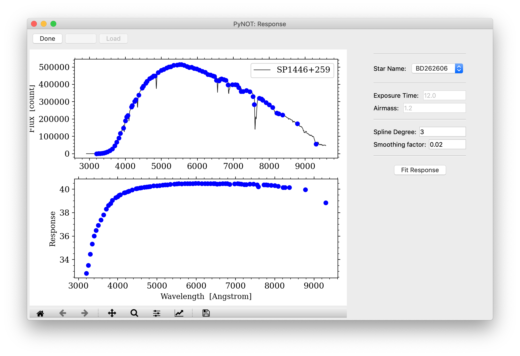
pynot response. The wavelength-calibrated,
1-dimensional spectrum of the star BD262606 is shown in black. The blue dots mark the calculated obesrved flux in the same
wavelength bins as the available measurements of absolute flux of the standard star.
Fitting the response
It's important to pay attention to absorption or emission features in the spectrum as these depend on the spectral resolution and therefore do not represent the exact flux in the given wavelength band. These should masked out. This can be done by clicking on a given blue point. It will then turn into a red cross, indicating that it will no longer be used when fitting the response function. Clicking on that point again will toggle it back on. (This part of the interface is sometimes a bit lagging, I apologize.)When you have filtered out all the bad points, you can fit the response function by clicking the "Fit Response" button. This is done using a combination of spline fitting of a variable degree and a smoothed and clipped interpolation. For the best result, the smoothing parameter should be of the order of the uncertainty on the measured points.
The best fit response function will show up as a solid blue line, as seen in Fig. 2.
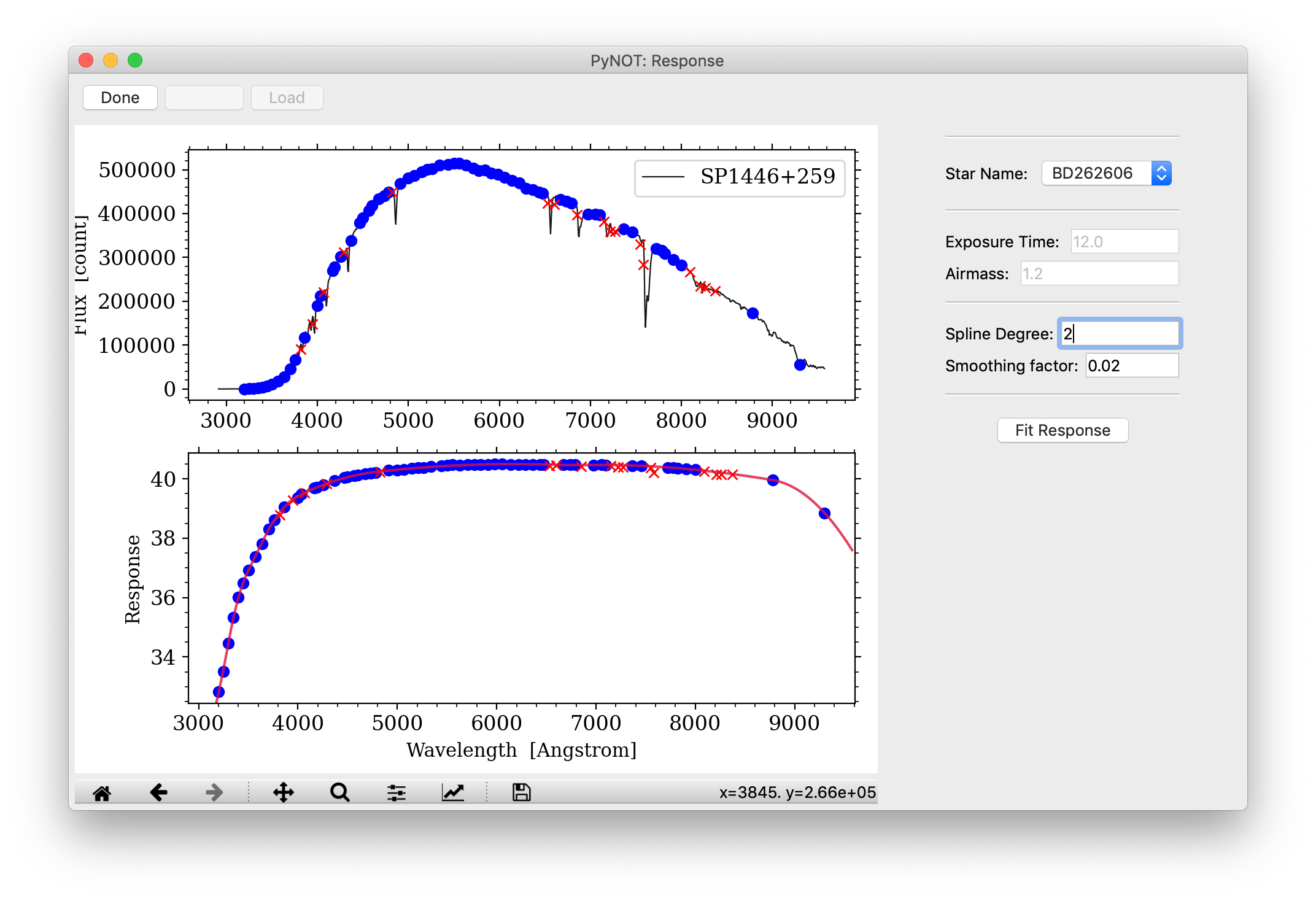
pynot response. The response function has
been fitted using a smoothing spline of variable degree. The best-fit response function is shown as the red solid line in the
bottom panel.
When you are happy with the fitted response curve, you can save it to a file by clicking the "Done" button in the upper left corner. This will save the response function to a FITS table by default, which can be used in the PyNOT tasks flux1d and flux2d to apply the flux calibration to a processed science spectrum. The response function converts the observed counts into spectral flux density per wavelength unit: \({\rm erg\ s^{-1}\ cm^{-2}\ Å^{-1}}\).
List of standard stars
The list of currently available standard stars is given here:- bd174708
- bd262606
- bd332642
- bd75325
- eg21
- feige110
- feige34
- gd153
- gd50
- gd71
- hd19445
- hd84937
- hd93521
- he3
- hiltner600
- ltt3864
- wolf1346
Example Syntax
pynot response
Full example of command line syntax:
pynot response [-h] [-o OUTPUT] [input]
Overview of parameters
Optional Arguments:- input
- Input filename of 1D spectrum of flux standard star
- --output (-o): ''
- Output filename of response function